cbrad: Computing variance

Given a list of n numbers $x_1,x_2,...,x_n$ , the variance is defined as

$\frac{1}{n}\sum_{i=1}^n{\left(x_i - \bar{x}\right)^2}\quad\quad\quad\text{(1)}$

where $\bar{x}$ is the arithmetic mean.

$\bar{x} = \frac{1}{n}\sum_{i=1}^n{x_i}$

Expression 1 stated in words is the average squared difference of each data point from the mean. Implemented as an algorithm, this requires two passes over the data set. The first to calculate the mean and the second to sum the squared differences.

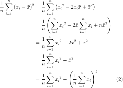
Let's derive the more commonly used expression for variance.

$\begin{align*} \frac{1}{n}\sum_{i=1}^n{\left(x_i - \bar{x}\right)^2} & = \frac{1}{n}\sum_{i=1}^n{\left({x_i}^2 - 2x_i\bar{x} + \bar{x}^2\right)} \\ & = \frac{1}{n}\left(\sum_{i=1}^n{x_i}^2 - 2\bar{x}\sum_{i=1}^n{x_i} + n\bar{x}^2\right) \\ & = \frac{1}{n}\sum_{i=1}^n{x_i}^2 - 2\bar{x}^2 + \bar{x}^2 \\ & = \frac{1}{n}\sum_{i=1}^n{x_i}^2 - \bar{x}^2 \\ & = \frac{1}{n}\sum_{i=1}^n{x_i}^2 - \left(\frac{1}{n}\sum_{i=1}^n{x_i}\right)^2 && \text{(2)} \end{align*}$

This only requires a single pass over the data set, computing the incremental sum of the values and the incremental sum of their squares. However, if the terms in the subtraction are large and close enough, catastrophic cancellation can occur. Essentially the precision of the floating point representation is exceeded, yielding unacceptable results. See Algorithms for calculating variance and Theoretical explanation for numerical results for examples (they are calculating the sample variance which is slightly different). More detailed information on catastrophic cancellation can be found in What Every Computer Scientist Should Know About Floating Point Arithmetic (1991).

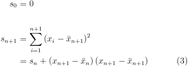
A more numerically stable (but computationally expensive) single pass algorithm was published by Knuth in The Art of Computer Programming, volume 2. Define $\bar{x}_n$ and $s_n$ as the mean and sum of squared differences of the the first n values respectively.

$\begin{align*} s_0 & = 0\\ \\ s_{n+1} & = \sum_{i=1}^{n+1}\left(x_i-\bar{x}_{n+1}\right)^2\\ & = s_n + \left(x_{n+1}-\bar{x}_n\right)\left(x_{n+1}-\bar{x}_{n+1}\right)\quad\quad\quad(3) \end{align*}$

For m > 0 values, the variance is then $\frac{s_m}{m}$ .

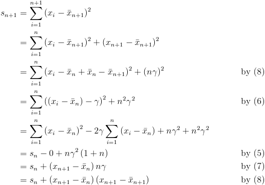
Derivation of Equation 3
This is really just a more verbose version of one-pass algorithm to compute sample variance. First up is the running mean.

$\begin{align*} \bar{x}_0 & = 0\\ \\ \bar{x}_{n+1} & = \frac{n\bar{x}_n + x_{n+1}}{n+1}\\ & = \frac{\left(n+1\right)\bar{x}_n-\bar{x}_n+x_{n+1}}{n+1}\\ & = \bar{x}_n + \frac{x_{n+1}-\bar{x}_n}{n+1} && \quad &&& (4)\\ \end{align*}$

If you think of the mean visually i.e. a horizontal line through the data on a scatter plot, then it is intuitive that the sum of the distances between each point and the mean is zero.

$\sum_{i=1}^n\left(x_i-\bar{x}_n\right) & = \sum_{i=1}^nx_i-n\left(\frac{1}{n}\sum_{i=1}^nx_i\right)=0\quad\quad\quad(5)$

Now define $\gamma$ as the difference of consecutive incremental means, along with a few useful variations.

$\begin{align*} \gamma & = \bar{x}_{n+1} - \bar{x}_n && \quad &&& (6)\\ \\ \gamma & = \bar{x}_n + \frac{x_{n+1}-\bar{x}_n}{n+1} - \bar{x}_n && &&& \text{by (4)}\\ \gamma & = \frac{x_{n+1}-\bar{x}_n}{n+1} \\ \left(n+1\right)\gamma & = x_{n+1}-\bar{x}_n && &&& (7)\\ \\ x_{n+1}-\bar{x}_{n+1} & = x_{n+1}-\bar{x}_n+\bar{x}_n-\bar{x}_{n+1} \\ & = \left(n+1\right)\gamma-\gamma && &&& \text{by (7, 6)} \\ & = n\gamma && &&& (8)\\ \end{align*}$

The pieces are now all in place to derive equation 3.

$\begin{align*} s_{n+1} & = \sum_{i=1}^{n+1}\left(x_i-\bar{x}_{n+1}\right)^2\\ & = \sum_{i=1}^{n}\left(x_i-\bar{x}_{n+1}\right)^2 + \left(x_{n+1}-\bar{x}_{n+1}\right)^2\\ & = \sum_{i=1}^{n}\left(x_i-\bar{x}_n+\bar{x}_n-\bar{x}_{n+1}\right)^2 + \left(n\gamma\right)^2 && \quad &&& \text{by (8)}\\ & = \sum_{i=1}^{n}\left(\left(x_i-\bar{x}_n\right)-\gamma\right)^2+n^2\gamma^2 && &&& \text{by (6)}\\ & = \sum_{i=1}^{n}\left(x_i-\bar{x}_n\right)^2 -2\gamma\sum_{i=1}^{n}\left(x_i-\bar{x}_n\right)+n\gamma^2+n^2\gamma^2\\ & = s_n-0+n\gamma^2\left(1+n\right) && &&& \text{by (5)}\\ & = s_n+\left(x_{n+1}-\bar{x}_n\right)n\gamma && &&& \text{by (7)}\\ & = s_n+\left(x_{n+1}-\bar{x}_n\right)\left(x_{n+1}-\bar{x}_{n+1}\right) && &&& \text{by (8)} \end{align*}$

cbrad

Sunday, March 21, 2010

Computing variance

No comments:

Blog Archive

Subscribe

Labels